If you want to highlight a cell in Excel based on its value, it’s pretty straight forward: Just choose Conditional Formatting from the Home ribbon. But what if you want to highlight the entire row based on the value in just one of the cells? We’ll use Conditional Formatting here too, but with a slightly different approach than we’re used to.
This is what we want: Choose one of the names in the table below and highlight the entire row for each occurence of that name.
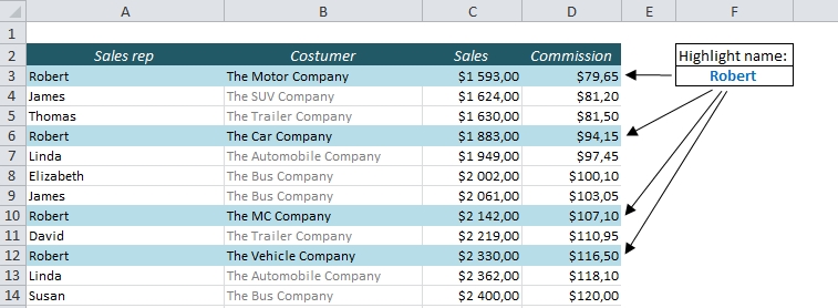

First, let’s look at the criterion field. This is where we choose which rows we want to highlight. In my example, I’ve chosen Robert, so every row that has the name Robert in column A will be highlighted. You might want to create a drop-down menu in this field, but it’s not necessary. Check out this post to learn how to create a drop-down list in 3 minutes (opens in a new tab).
Conditional Formatting checks for a TRUE or FALSE, and formats the cells that are TRUE. We want to check if the value in column A is equal to the value in our name field (F3).
The statement =A2=F3 will return TRUE if we choose Robert in F3, and FALSE for any other name.
In order to make this work for the entire row we have to lock the column reference A (we are not interested in the values in B, C and D) and of course, the reference to the criterion in F3. This is the formula we will use for the Conditional Formatting:
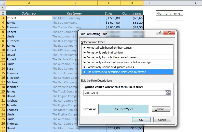
=$A3=$F$3
Let’s do it: Select all the cells in the table, click on Conditional Formatting from the Home ribbon and choose New Rule (Shortcut: Alt > H > L > N). Choose “Use a formula to determine which cells to format” and type the formula in the formula field.
Done! Choose a name in F3, and all the rows with that name will be highlighted!
More on Conditional Formatting:
- Hide Future Dates in Excel with Conditional Formatting
- How to Find Duplicates and Triplicates in Excel
- The Easiest Way to Hide Zeros in Excel
- Create a Search Box in Excel without VBA
Are you using a non-English version of Excel? Click here for translations of the 140 most common functions in 17 different languages:
Catalan
Czech
Danish
Dutch
Finnish
French
Galician
German
Hungarian
Italian
Norwegian
Polish
Portuguese (Brazilian)
Portuguese (European)
Russian
Spanish
Swedish
Turkish
Hi.
Great article.
maybe you can help with my problem, that is similar to your explanation.
I have a matrix that each cell is composed by a function of two parameters (two columns). The formula is “=COUNTIFS(T2:T99,”15″,V2:V99,”14″)”, so it’s counts when in one column we receive 15 and in the other 14.
For instance, I receive the number 3 – so I have three rows that match.
I want, when I select the cell with the number 3 (that I receive from the formula) it will highlight the relevant rows..
could you help me??
Thank you
Thank you!
It should work if you highlight the columns T and V, select Conditional Formatting, and use this function:
=AND($T1=15,$V1=14)
I’m attempting to create a unit conversion chart (see link below). I have all my data and one of the drop down boxes for the different categories complete (Ex. Temperature, Area, Volume, etc…). How can I add the second and third drop down lists so that only it only shows the corresponding unit to the category? For example, Temperature only needs to show Celsius, Farenheit and Kelvin…
https://www.google.com/?gws_rd=ssl#q=conversion+calculator
Thanks
Justin
Maybe this article can help: http://easy-excel.com/dynamic-drop-down-in-excel/