Is there an easy way to locate and highlight duplicates in a list in Excel?
If you just want to remove the duplicates, the easiest way is to use the Advanced Filter or the built-in Remove Duplicates feature on the Data ribbon, but what if you want to find the duplicates in the list, keep them and highlight them with a different colour? That almost sounds like a job for a professional Excel consultant, but there’s no need for that – you can easily do it yourself! I’ll show you one easy way and one super-easy way:
First, the super-easy way:
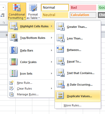
Select the cells you want to check, go to the Home Ribbon, choose Conditional Formatting and select Highlight Cell Rules > Duplicate Values.
Then, the easy way
If you only want to locate duplicates, the super-easy way above is the right way to do it. But sometimes we want to make it more dynamic: If we want to be able to choose between highlightning duplicates, triplicates or quadruplicates, i.e. two, three or four occurrences of the same piece of data, we need another approach: Conditional Formatting with a formula.
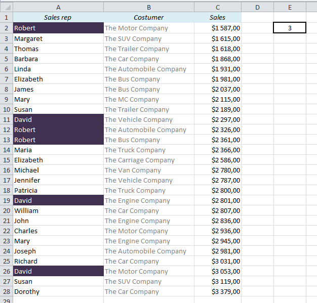
First, let’s find out how to count the number of occurences in a list. In my example below I have 27 rows of data, with names in the range A2 to A28. In A2 we find the name Robert, so if we want to find out how many times Robert appears in the list, we can use this formula: =COUNTIF($A$2:$A$28,A2). In this example the formula will return 3.
We will use almost the same formula in Conditional Formatting: As you might already know, Conditional Formatting uses Boolean logic, which means that it checks whether or not a statement is TRUE, and formats the cells that return TRUE. First, let’s see how our formula works when we put it in the worksheet. We use the same formula as above, only with “=1”, “=2” or “=3” in the end, and we will get TRUE or FALSE for each statement. In this example, for Robert, the statement is true for “=3”.

So, let’s put the formula into Conditional Formatting, with one small adjustment: Instead of hard-coding the value after the equal sign (1,2,3 etc.) we’ll use a cell reference. I will have my reference in cell E2.
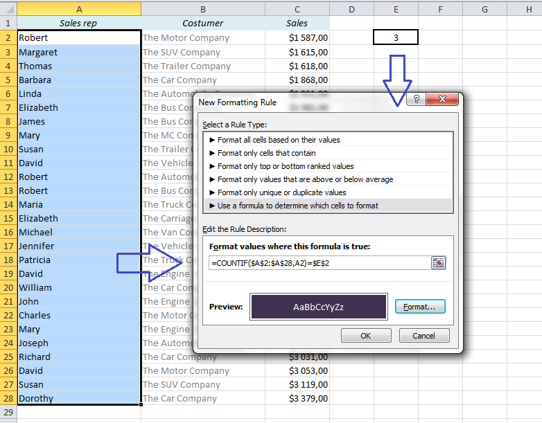
Select the cells you want to include in the search (A2:A28 in this example), go to the Home Ribbon and choose Conditional Formatting > New Rule. Select “Use a formula to determine which cells to format” and type this formula into the formula field:
=COUNTIF($A$2:$A$28,A2)=$E$2
Note that the range A2:A28 and the reference to E2 (number of occurrences) have to be locked with dollar signs (shortcut: F4). The criterion, A2, must remain unlocked.
The result: All the triplicates are highlighted. If you change the value in E2 to 2, you will get the duplicates instead, and if you change it to 1, all the unique values will be highlighted.
If you want to highlight all the recurrences of a value (both duplicates, triplicates, quadruplicates etc.), you can use this formula instead:
=COUNTIF($A$2:$A$28,A2)>1
More easy tricks with Conditional Formatting:
- Create a Search Field in Excel in 5 minutes
- Highlight an Entire Row in Excel Based on One Cell Value
- The Easiest Way to Hide Zeros in Excel
- Hide Future Dates in Excel with Conditional Formatting
Are you using a non-English version of Excel? Click here for translations of the 140 most common functions in 17 different languages:
Catalan
Czech
Danish
Dutch
Finnish
French
Galician
German
Hungarian
Italian
Norwegian
Polish
Portuguese (Brazilian)
Portuguese (European)
Russian
Spanish
Swedish
Turkish
Strangely none of this work for me except the predefined rules in excel. When I type a formula excel doesn’t mind it at all. I really don’t know why.
So my case is as follows:
I’ve got a column with values that ideally should come in couples. But there a some of them that are unique and some that are appearing more than twice. The ones that a unique are unnecessary and will be deleted but the others will receive special attention.
Is there any remedy to it, I will be happy to receive any suggestions!
You can use Conditional formatting with this formula: =COUNTIF($A$2:$A$1000,A2)=1
This will highlight the unique values. Or you can do as described above, and change the value in E2 to 1.
(You might have to replace the comma with a semi-colon, depending on your local settings.)
I have three columns, separated by other data, that I would like to compare and highlight triplicates. I have tried your method above and it works except for the very top row of the three columns. Is there any way to fix that?
Thanks
Is it possible that the formula in Conditional Formatting doesn’t cover the whole range? If that’s not the case, I have no idea… You’re welcome to e-mail it to me (a.danielsen -(at)- gmail.com), and I can try to find the error.
Actually I just figured it out. Thanks for your help.
You said ‘super easy’ and I truly didnt believe you but I was super wrong. That was brilliant thank you.
HI, good day !
I have a column with series of truck numbers. I need to high light their second arrival in one color and the third in another color. Your suggestion does not work to me as i can not name any truck number by A2. any other easy way to do this ?
many thanks
Senna
htadis@gmail.com
Using Excel 2013 I get an error with your formula – if i type it without the ,A2 it says I have too few arguments, if I type it with the ,A2 part – it says that I have an error in the formula and should check it.
My case is the following – I have a column (F actually) with 4037 values and I need to find out which of the them is repeated 4 or more times.
When i copy this formula: =countif($a$2:$a$25,$a$2)>2
it highlights the entire column rather than just the cells once a triplicate arrives – what am i doing wrong?
It could be because of the dollar signs around the last argument. Does it work with =COUNTIF($A$2:$A$25,A2)>2 ?
How annoying that Audun does not answer the two people who have the same issue I have, but answers everyone else. It is pointless to type in a formula when one can just use the Find function for their dupes. Sure – it would be annoying to do this for large amounts of data, but my frustration is that I DON’T KNOW what the values are that are dupes, triplicates etc, and that is what I need excel to find for me. What does the formula look like without a criterion????
Hi, any idea on an Excel of championship results that contains four columns of names and four of points and I have to find and highlight all the names that are triplicates (those qualify for an elite championship)? What criterion should I set? The “A2” does not work.
Thank you SO much for this super easy way. A big help for me!!!
i have only 1 column. from a1 to a50 for example.
how to highlight triplicate from a1 to a50.
thank you.
Try Conditional formatting with this formula:
=COUNTIF($A$1:$A$50,A1)=3
this works… mostly. But when highlighting triplets, it only highlights 2 of the 3 and not the one that’s furthest down on the list. Likewise, if I highlight duplicates, it only highlights the highest one on the list.
thanks for the help!
Be sure to include all the rows in your formula: If you have a range from A1 to A200, for example, the formula in Conditional formatting should be
=COUNTIF($A$1:$A$200,A1)=$E$2
(Cell E2 is where you have the criterion; 2 for duplicates, 3 for triplicates etc)
Need a formula of repetation of a name three times in a sheet by changing color of the said column
Pingback: Compare List Excel – Almazrestaurant