How can we calculate the grades (for example A-F) in Excel if we have the test results as numbers? In the example below, a score of 90% or higher is an A, 80-89% is a B, 70-79% is a C, 65-69% is a D and less than 65% is an F.
The first thing we should do is to organize this information in a lookup table:
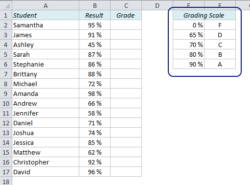
It is important that the table is sorted in ascending order, with the numbers to the left and the letters to the right. Now we can use the VLOOKUP function to look up the value in the left column and return the value in the right column.
The VLOOKUP function looks for a value in a table and returns another value on the same row in that table. Sometimes you want to look for an exact match, but in this case we want to find an approximate match, ie. if the score is greater than or equal to 70%, but less than 80%, the student gets a C.
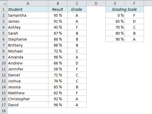
Let’s type a formula in C2 and see which grade Samantha got:
=VLOOKUP(B2,$E$2:$F$6,2)
The first argument in this formula, B2, is Samantha’s result, in percent. The second argument, $E$2:$F$6, is the lookup table. Don’t forget the dollar signs (shortcut: F4) to lock the reference in order to be able to copy the formula down. The third argument, 2, is the number of the column that has the value we’re looking for. VLOOKUP also allows for a fourth argument; exact match or approximate match. In this case we want an approximate match, which is default for this function, so we don’t have to specify it in the formula.
Copy the formula down, and the grade report is done!
But what if you are not allowed to sort the grading scale and it looks like this:
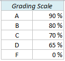
Neither VLOOKUP nor INDEX+MATCH will work here. We have to use a nested IF-function.
=IF(B2>$F$2,$E$2,IF(B2>$F$3,$E$3,IF(B2>$F$4,$E$4,IF(B2>$F$5,$E$5,$E$6))))
Explanation:
If B2 (95%) is greater than F2 (90%), return the value in E2 (A)
If not, check if B2 is greater than F3 (80%) and return the value in E3 (B)
If not, check if B2 is greater than F4 (70%) and return the value in E4 (C)
If not, check if B2 is greater than F5 (65%) and return the value in E5 (D)
If not, return the value in E6 (F)
I would not recommend this solution unless it’s absolutely necessary. It’s difficult to write the formula, especially if you have a larger table than in this example, and the risk of error is a lot higher than if you use the VLOOKUP method.
More on Lookup techniques in Excel:
- How VLOOKUP can get you in trouble and how to solve it
- How to create a dynamic chart in Excel
- Create a Search Box in Excel without VBA
Are you using a non-English version of Excel? Click here for translations of the 140 most common functions in 17 different languages:
Catalan
Czech
Danish
Dutch
Finnish
French
Galician
German
Hungarian
Italian
Norwegian
Polish
Portuguese (Brazilian)
Portuguese (European)
Russian
Spanish
Swedish
Turkish
You could also manipulate the scale and then use INDEX/MATCH. Leave the grading scale as is F2:F6 and put the following in G2:G6:
100%
89%
79%
69%
64%
Then use the formula:
=INDEX($E$2:$E$6,MATCH(B2,$G$2:$G$6,-1))
An equal sign is needed immediately after each of the greater than sign in =IF(B2>$F$2,$E$2,IF(B2>$F$3,$E$3,IF(B2>$F$4,$E$4,IF(B2>$F$5,$E$5,$E$6))))
to compute the grade accurately for marks such as 90, 80, 70, and 65. Morin’s INDEX/MATCH works flawlessly.
Correct me if I made mistakes.
I need your help on the issues concerning this kind of calculations
In our country we have this kind of Grading
0 – 14 is F9
15 – 29 is P8
30 – 39 is P7
40 – 49 is C6
50 – 59 is C5
60 – 69 is C3
70 – 84 is D2
85 – 99 is D1
F stands for Failure
P stands for Pass
C stands for Credit
D stands for Division
I request you to help me in grading using that type of grading because I tried it out with the method up but I failed.
I want to put those gradings to Report Cards
Thank you
Nicholas
I would make a table with 3 columns: The same two as in my example above, and one additional column for the categories Failure, Pass, Credit and Division, like this:
Please, following the table above, I wish to add another another Column for positioning. How can the formula for calculating position to written?
Thanks!
Please, following the table above, I wish to add another another Column for positioning, i.e. 1st, 2nd, 3rd, 4th… after the grade. How can the formula for calculating position to written?
Thanks!
Hi Audun,
I’ve an exemplary grade dataset as below:
sn physics chemistry biology english math
1 45 56 45 78 45
2 12 5 78 78 78
3 45 45 45 45 42
4 78 45 78 78 78
5 78 78 78 78 78
6 45 78 87 78 45
7 56 87 78 87 95
8 30 78 79 78 78
9 78 78 30 78 28
10 45 45 45 45 78
11 89 78 45 78 84
12 45 78 4 12 85
13 12 45 78 45 78
14 45 78 78 56 94
15 78 45 78 54 64
If a student gets less than 40 in any of the subjects in a class, then the student fails and gets ‘No Division’. In other cases, the ‘passed’ students are categorized based on aggregated% as: >=80% (Distinction), >=60% (First Division), >=45% (Second Division), <45% (Third Division)
In such cases, I need one column that shows whether the student passed or failed and another column shows the Division for those who passed and 'No division' for those who failed. How can we do? Your support will be helpful.
Regards.
Basan Shrestha
Hi Basan,
You can use the MIN function to test whether any of the values are below 40:
If you have the scores in columns B to F, try this in column G:
=IF(MIN(B1:F1)<40,"No Division",[Value if true])
For "Value if true" you can use the VLOOKUP formula described in the article, with the lookup value expressed as the average of the columns.
how are you mr, I need more your helpful to arrange subject grades start F up to A
how to do the calculation …..with bellow condition….
Marks Grade
>=800 A+
>=750 A
>=700 A-
>=650 B+
>=600 B
>=550 B-
>=500 C+
>=450 C
>=400 D
>=360 P
<360 F
hello
i want to ask about adding letter grades and average in excel with VLOOKUP.
thank you
91
73
77
89
80
92
45
79
87
81
Please help me to grade
90-100 A
85-90 B
70-85 C
Below 70 F
Please if I have the following data,
1
3
2
4
Which formula can I use to select the smallest two numbers in excel
Thank you
thanks for your article, I am currently using gradecalculatorpro.com to calculate the grade, and I am searching for something to help me to calculation off-line. thanks for the solution, Now I can calculate grade on Excel.