In many situations you collect data every day (sales figures, stock prices etc.) for weeks, months and years, while all you want to show in the chart is the last week or two. I’ve seen many people spending a lot of time updating the chart manually every day, so here I will show you how you can make a dynamic chart that always shows the last 7 days. Of course, you can use the same technique for any number of days, weeks or months.
First, let’s get an overview of what we have and what we want:
What we have:
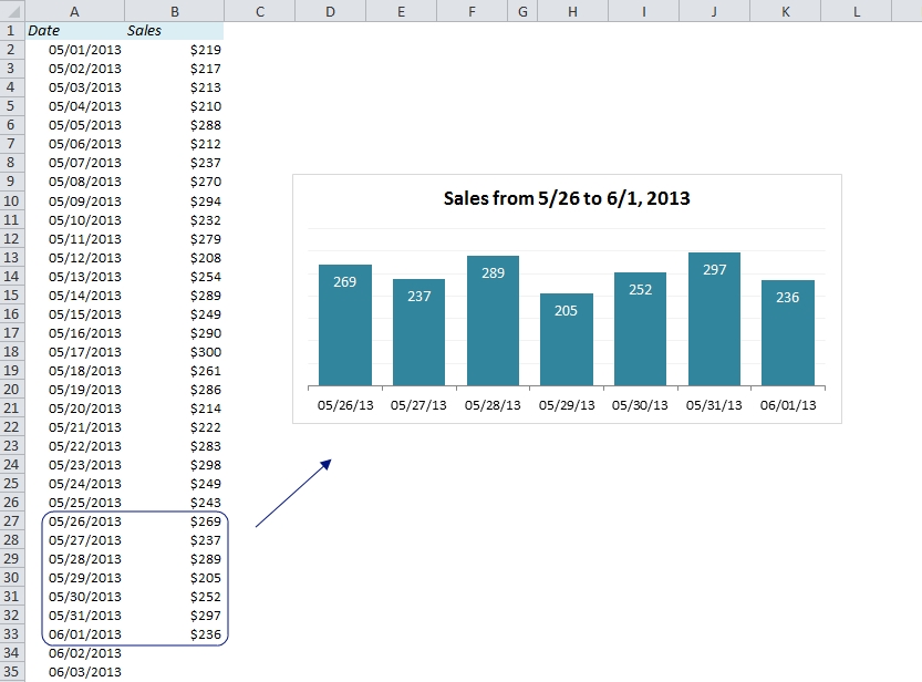
- A table in column A and B with daily sales figures with one amount for each day.
What we want:
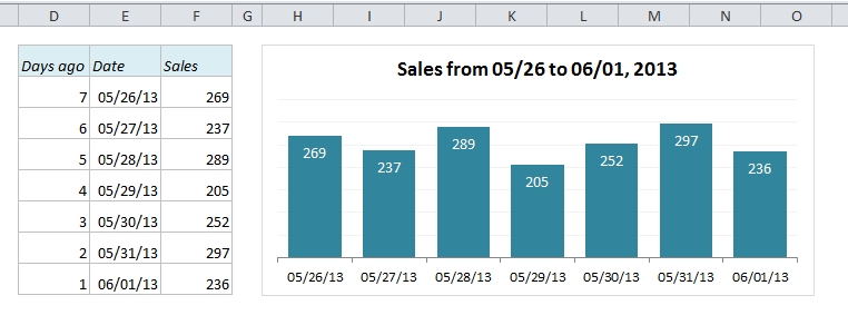
- A dynamic chart that displays the sales for the past 7 days.
- A dynamic chart title, e.g. “Sales from 5/26 to 6/1, 2013”
Step 1: Create a dynamic table
The chart will get its data from this new table, not the large table in column A and B.
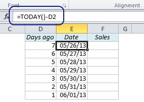
The first column in the new table, Column D, is called “Days ago”. This number is used to calculate the date in column E. With the formula =TODAY()-D2 copied down it will always return today’s date minus 7, 6, 5 etc, so when you open the file tomorrow, the dates will have updated.
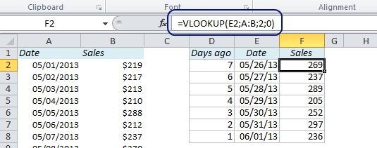
In the F column we will find the sales figures for these dates using a VLOOKUP formula.
The formula =VLOOKUP(E2,A:B,2,0) works like this:
- Look up what? E2
- Look up where? A:B (Columns A and B)
- Return what? 2 (the value in the second column)
- …and the zero means Excact match
Step 2: Create a chart title
The text we want is “Sales from 5/26 to 6/1, 2013”, with the dates changing automatically every day.
This text has 4 elements:
“Sales from “ & 5/26 & ” to “ & 6/1, 2013, and that’s how we will write the formula as well, only replacing the hard-codes dates with cell references. Choose any cell in the worksheet for this formula.
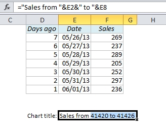
=”Sales from “&E2&” to “&E8
Unfortunately, the result of this formula is “Sales from 41420 to 41426”.
We have to tell Excel to format these numbers as dates. So, we wrap a little function around the cell references E2 and E15:
TEXT(E2,”m/d”). This converts the number of the date (41420) to the date format m/d, or 5/25.
TEXT(E8,”m/d, yyy”). This converts the number of the date (41426) to the date format m/d, yyy, or 6/1, 2013.
Here’s the final formula for our dynamic chart title:
=”Sales from “&TEXT(E2,”m/d”)&” to “&TEXT(E8,”m/d, yyy”)
…which gives this result: Sales from 5/26 to 6/1, 2013
Step 3: Create the chart
This is the easy part! Select the Date column (E) and the Sales column (F), including the header, and choose a chart type from the Insert ribbon.
Excel assumes that we want the Chart title to be the same as the header in column F; “Sales”. To change it, simply click once on the title, type an Equal Sign (=) and click on the cell where we wrote the title formula.
Finally, hide the chart title formula under the chart using cut and paste (Ctrl+X > Ctrl+V) and apply some formatting to make the report look good.
More articles on Excel Charts:
- 5 Easy Steps to Make Your Excel Charts Look Professional
- Excel Line Charts: Why the line drops to zero and how to avoid it
Are you using a non-English version of Excel? Click here for translations of the 140 most common functions in 17 different languages:
Catalan
Czech
Danish
Dutch
Finnish
French
Galician
German
Hungarian
Italian
Norwegian
Polish
Portuguese (Brazilian)
Portuguese (European)
Russian
Spanish
Swedish
Turkish