EDIT: If you are using Excel 2019 or Office 365 you can use the TEXTJOIN function to solve this problem. Click here for the new article:
How to Join Text from Several Cells in Excel using TEXTJOIN
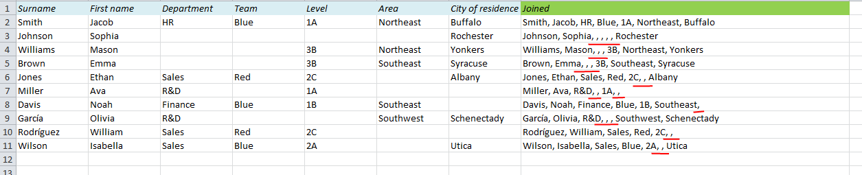
Unclean data can cause a lot of problems in Excel. In this post I will show how you can join data from different columns with a comma between them. That’s the easy part. The problem occurs when you have empty cells in your data, like in the table below. The result of the first row looks fine, but if you look at the rows with empty cells, you get too many commas:
Joining the strings
First, let’s look at how we join the strings. We’ll deal with the commas later.
There are two ways to do this, either with the CONCATENATE function, or with the Ampersand (&)operator. With Ampersand, you start with the first element, add the the “&”, type the next, add another “&”, and so on:
=A2&B2&C2&D2&E2&F2&G2
The result of this formula is “SmithJacobHRBlue1ANortheastBuffalo”, so we have to add the commas (and a space) between the cell references. The comma+space is a text string, and has to be wrapped between double quotes:
=A2&”, “&B2&”, “&C2&”, “&D2&”, “&E2&”, “&F2&”, “&G2
The second way to join cells is the CONCATENATE function. Instead of all the Ampersand symbols, you simply start with the function name, and separate the elements with a comma (or semicolon for some international Excel users):
=CONCATENATE(A2,”, “,B2,”, “,C2,”, “,D2,”, “,E2,”, “,F2,”, “,G2)
Removing the extra commas
As we saw on the picture above, this works fine as long as there are no empty cells in the raw data. However, that is rarely the case, and if we don’t want the extra commas in our result, we have to adjust our formula a little bit.
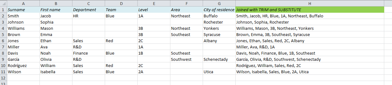
The TRIM function in Excel can be used to get rid of excess spaces in a text string. Unfortunately, there is no function that removes excess commas, so we have to start with a string with spaces instead of commas, then remove excess spaces, and finally replace the spaces with commas. Here are the 3 steps:
- Step 1: Join the cells with a space between each cell
(The CONCATENATE part) - Step 2: Wrap the TRIM function around it to get rid of excess spaces
- Step 3: Wrap the SUBSTITUTE function around that to replace the spaces with commas
We end up with this formula: =SUBSTITUTE(TRIM(CONCATENATE(A2,” “,B2,” “,C2,” “,D2,” “,E2,” “,F2,” “,G2)),” “,”, “)
If you are using Excel 2019 or Office 365 you can use the TEXTJOIN function to solve this problem. Click here for the new article:
How to Join Text from Several Cells in Excel using TEXTJOIN
More on text functions:
- How to Join Text from Several Cells in Excel using TEXTJOIN
- Convert text to number with formula
- Create random text strings and line breaks with the CHAR function
- Use Excel to Count Words
- Bahttext
- Use Excel to count characters
Are you using a non-English version of Excel? Click here for translations of the 140 most common functions in 17 different languages:
Catalan
Czech
Danish
Dutch
Finnish
French
Galician
German
Hungarian
Italian
Norwegian
Polish
Portuguese (Brazilian)
Portuguese (European)
Russian
Spanish
Swedish
Turkish
Hi
I tried the solution you posted above on a file I have, but it didn’t work.
Is it ok if I send you the file?
Best regards
Jona
If you have your data in A2 to G2, this should work:
=SUBSTITUTE(TRIM(CONCATENATE(A2,” “,B2,” “,C2,” “,D2,” “,E2,” “,F2,” “,G2)),” “,”, “)
But you might want to try to type the formula instead of copying it. The quotes can cause problems.
Also, if you use a non-English version, you might need to replace the commas between the formula arguments with semi-colons.
My problem was that some of the text in my cells comprised of multiple words and I needed commas between the cells as opposed to the words.
My need was actually merging an address: business name, suite/level/unit, street address, suburb, postcode.
I used the following solution:
=concatenate(IF(A2=0, “”,A2&”, “),IF(B2=0,””,B2&”, “),IF(C2=0,””,C2&”, “),IF(D2=0,””,D2&”, “),IF(E2=0,””,E2))
Concatenate combines all the data.
The IF statements checks cell A2. If there is no value (=0) in the cell it returns “”. This returns nothing and doesn’t generate a space at all. If there is a value in the cell it returns the value of A2 and includes “, ” as a suffix.
Repeat for the remainder of cells you would like to include and leave the suffix out of the last IF statement.
I have updated this:
=concatenate(IF(A2=””, “”,A2&”, “),IF(B2=””,””,B2&”, “),IF(C2=””,””,C2&”, “),IF(D2=””,””,D2&”, “),IF(E2=””,””,E2))
I replaced 0 with “” to identify a blank cell as oppose to a nil value.
Oh how I wished one of these would have worked. I tried both.
I need to concatenate columns H2, I2, J2 and K2 into one text string, separated by commas only (no space).
First I tried the original post solution of =SUBSTITUTE(TRIM(CONCATENATE… but this just replaced all the spaces IN the cells with commas as well.
Then I tried Timothy’s formula, which looked like:
=CONCATENATE(IF(H2=””, “”, H2&”,”),(IF(I2= “”, “”, I2&”,”),(IF(J2=””, “”, J2&”,”),(IF(K2=””, “”, K2)))))
and got #VALUE!. Where’s my error…?
Timothy! You do not know how much this has saved me! I have been on this for two days! Thank you!
Just what I was looking for, thank you very much!
Thanks so much – this solved most of my problem. Now I have a dangling comma at the end of most of my lists, though, in every case where the last column is empty. Any ideas?
awesome topic ,i have a question.
how to use replace together with concatenate and trim
so i use this =TRIM(CONCATENATE((AC1,AD1,AE1)) it joint 3 cells and removed extra spaces ,but inside those cells i have a lots of / i, trying to replace them with space ,or maybe even just remove them?