How to Join Text from Several Cells in Excel using TEXTJOIN

I wrote an article a few years ago about how you can join data from different columns, and add a comma between each part. It was quite tricky, especially if we had some empty cells, so we ended up with a long formula with SUBSTITUTE, TRIM and CONCATENATE.

If you have Excel 2019 or Office 365, there is an easier way: The TEXTJOIN function.

Here’s the same dataset that I used in the previous article, and the result we want in the column to the right:

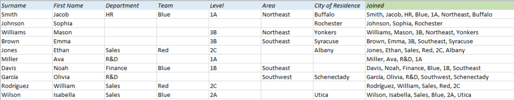
…and this is the formula we ended up using back then:

=SUBSTITUTE(TRIM(CONCATENATE(A2,” “,B2,” “,C2,” “,D2,” “,E2,” “,F2,” “,G2)),” “,”, “)

(CONCATENATE to combine the cells, TRIM to get rid of excess spaces, and SUBSTITUTE to remove excess commas)

It’s a lot easier now, if you have a new version of Excel. The TEXTJOIN function takes care of everything!

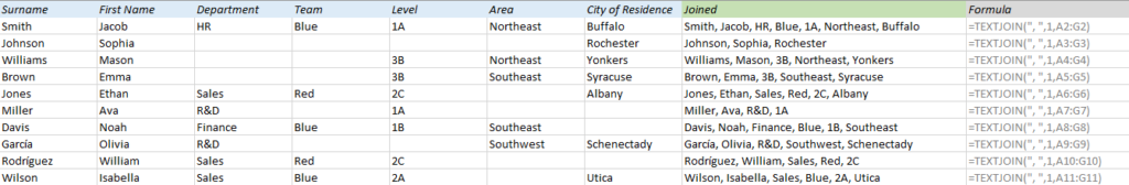
The TEXTJOIN function has three arguments: 1) Delimiter, 2) Whether or not you want to ignore empty cells in your range, and 3) the range.

In our example, we want to have a comma and a space as delimiter, so that’s what we type first, between double quotes (“”). Since we want to ignore empty cells, the second argument is 1 or TRUE (0 or FALSE if you want to include empty cells), and the last argument is the cells we want to join, A2:G2:

=TEXTJOIN(“, “,1,A2:G2)