Why it’s important to protect cells in Excel
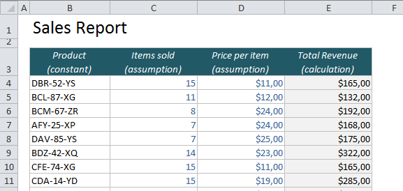
If you create an Excel report for someone, it is important that you somehow visualise which cells they are allowed to change, and which cells they should not touch. The common way to do this is to use a blue font for the assumptions, i.e. the values that can be changed.
Unfortunately, this is not always enough. Inevitably, someone will try to enter values into the calculation cells as well, and when they do, the whole report might be useless. We need to protect the cells from being tampered with, and the good news is that it takes less than a minute!
Using formatting to highlight assumptions
First, here’s how I use formatting (blue font) to show which values you are allowed to change. But remember, if it is still possible to make changes in all the other cells, someone will do it eventually! They might change a formula, and the report will never show the right results again!
How to protect cells in Excel in 3 easy steps
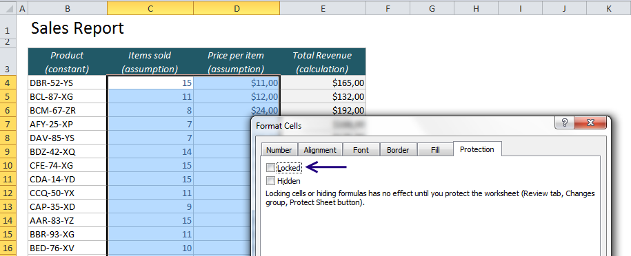
- If you just click on Protect Sheet on the Review Ribbon, all the cells will be protected. So, first we have to select the cells that should not be protected (the ones with the blue font)!
- Use the shortcut Ctrl+1 to open the Format Cells window. Select the Protection tab and uncheck Locked. Now, these cells will not be locked when we protect the sheet.
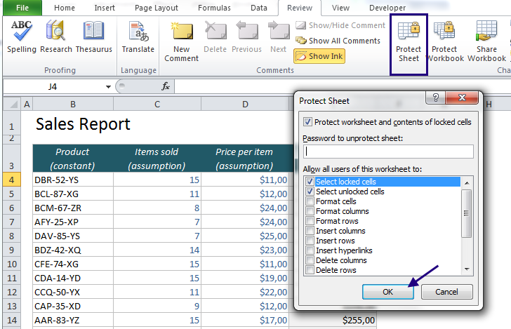
- Go to the Review Ribbon and choose Protect Sheet. If you want, you can protect it with a password, but that is usually not necessary. Just click OK, and everything but the assumption cells is locked!
To open the locked cells for editing, just click Unprotect (and the password if needed).
More tutorials:
- How to Find Duplicates and Triplicates in Excel
- Create a dynamic drop-down menu in Excel in 4 easy steps
- 5 Easy Steps to Make Your Excel Charts Look Professional
Are you using a non-English version of Excel? Click here for translations of the 100 most common functions.