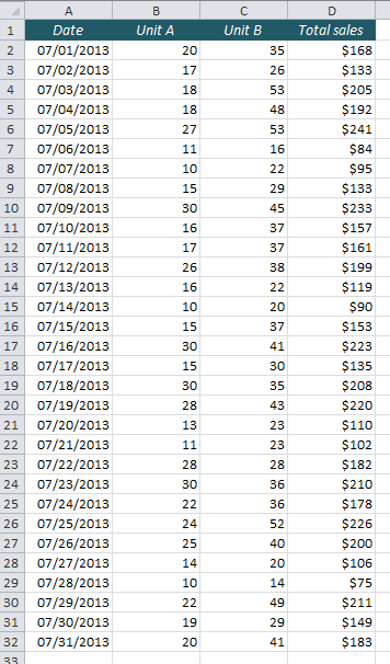
The picture to the right shows a table with some sales figures for July. There’s nothing wrong with the table as it is, but I find it very hard to read and make sense of it. There are just a lot of numbers and dates, and you can’t even distinguish between weekdays and weekends. If we could highlight the weekends (or weekdays) it would be a lot easier to read these numbers. In this example I want to highlight the Saturdays and Sundays. Here’s how we’ll do it:
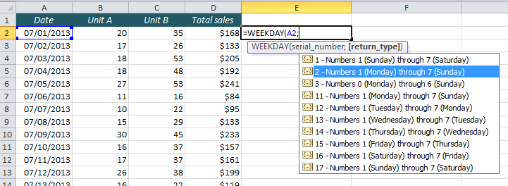
First, we have to think about how we can identify the Saturdays and Sundays. The WEEKDAY function returns a number from 1 to 7. There are several return type options (Sunday through Saturday, Monday through Sunday, Tuesday through Monday etc.), where each day corresponds to a certain number.
These are the numbers of the weekdays with return type 2:
- 1 – Monday
- 2 – Tuesday
- 3 – Wednesday
- 4 – Thursday
- 5 – Friday
- 6 – Saturday
- 7 – Sunday
As we see, every date in our table that returns a number that is larger that 5, (ie. 6 or 7) is a Saturday or Sunday, and should be highlighted. We will use Conditional Formatting, so we have to write a formula that returns a TRUE when the WEEKDAY is larger than 5:
=WEEKDAY($A2,2)>5
Note that I locked the column reference ($A2) to make sure that the Conditional Formatting only looks at the A column.
Select the whole table, Go to the Home ribbon, choose Conditional Formatting and click New Rule. Choose Use a formula to determine which cells to format, and type the formula in the field. Finally, click the Format button and choose font or background colour.
When you have done this a few times, you will be able to write the formula without even having to think, and this whole operation is done in seconds. This is the result:
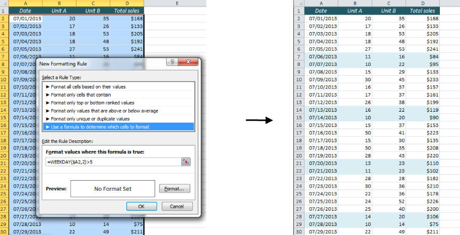
Of course, if you’d rather highlight Monday-Friday, you only have to change the last part of the formula: =WEEKDAY($A2,2)<6.
More on Conditional Formatting:
- Hide future dates with Conditional Formatting
- Highlight an Entire Row in Excel Based on One Cell Value
- The Easiest Way to Hide Zeros in Excel
- Create a Search Box in Excel without VBA
Are you using a non-English version of Excel? Click here for translations of the 100 most common functions.
To highlight Weekends using conditional formatting , is quite simple. You just need to enter 1 formula! How to make a dependent drop-down list in Excel . Find number of months between 2 dates in Excel .
Be careful with that function. You’ll notice that I used the value 2 as the WEEKDAY() function’s second argument. That’s important. Doing so uses Monday as the first day of the week, instead of Sunday – adjusting the values accordingly. This simple step simplifies the conditional formatting formula. The 5 component identifies the values 6 and 7 – which in this case are Saturday and Sunday. If you retain the default, the first day of the week is Sunday and this formula won’t work.
By the way! The best essay writing service – https://www.easyessay.pro/
Actually I have two work sheet
1 which is all days of week data while other one is 5 working days data
I have to merge both sheets but problem is date is not same
How can I handle it
Please help
Thanks