An Extra Column Means Trouble
If you want to find a value in a table in Excel, a simple VLOOKUP function is usually a good and easy way to do it. But you have to be careful – if you insert a new column in your table, the function might not work anymore, and we have to find another approach. Here’s why:
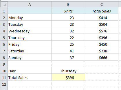
In the table below we have the Weekdays in Column A, Number of Units in Column B and Total Sales in Column C. To find the Total Sales for a specific weekday, we can use the VLOOKUP function:
=VLOOKUP(B10,A2:C8,3,0)
Explanation: The formula looks up the value in B10 (“Thursday”) in the array A2:C8 and returns the value in the 3rd column (column index number). The zero in the end of the formula means that we want an exact match.
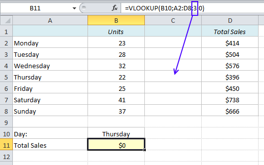
But what happens if we decide to insert another column between Units and Total Sales? The array reference will indeed update to A2:D8, but the column index number will still be 3. The formula will return the value in the new column, which is Zero!
Dynamic Column Reference
We need to make the column reference dynamic, in order for it to change whenever we insert a new column in the table. Let’s remove the extra column again and replace the hard-coded 3 with this MATCH function:
MATCH(A11,A1:C1,0)
Explanation: The formula looks up the value in A11 (“Total Sales”) in the array A1:C1 and returns the position of it. “Total Sales” is in the 3rd cell of this array (on the first picture). The zero in the end of the formula means that we want an exact match.
Let’s amend the VLOOKUP formula (assuming we have not yet inserted the new column):
Old formula: =VLOOKUP(B10,A2:C8,3,0)
New formula: =VLOOKUP(B10,A2:C8,MATCH(A11;A1:C1;0),0)
Does it work?
Let’s try to insert the new column again:
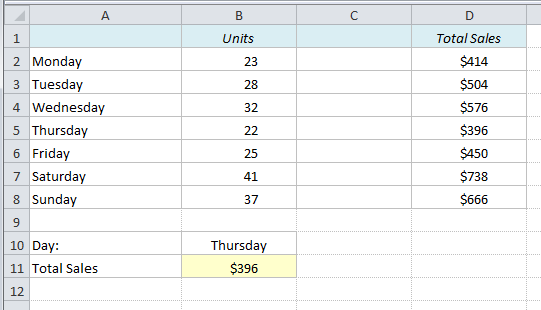
The value in B11 has not changed – it works!
INDEX & MATCH
Another approach to this problem would be an INDEX & MATCH combo.
=INDEX(B2:C8,MATCH(B10,A2:A8,0),MATCH(A11,B1:C1,0))
MATCH returns the relative positions, and INDEX returns the value in that cell intersection.
Some people prefer the INDEX & MATCH approach, but if you are already familiar with the VLOOKUP function, the VLOOKUP & MATCH approach described above is probably easier.
Note: If the lookup range is to the left of the lookup values, you must use the INDEX function. More on that in a future post!
What do you think? Do you prefer VLOOKUP or INDEX & MATCH? Feel free to make a comment below!
More Excel tricks:
- How to avoid #DIV/0 and other Error Messages in Excel
- How to Find Duplicates and Triplicates in Excel
- Yellow pop-up box when selecting cell in Excel
- How to Add All the Sums into an Excel Table in a Second
Are you using a non-English version of Excel? Click here for translations of the 100 most common functions.