Is it possible to create a search box in Excel, without using VBA?
Yes, and it’s easy!
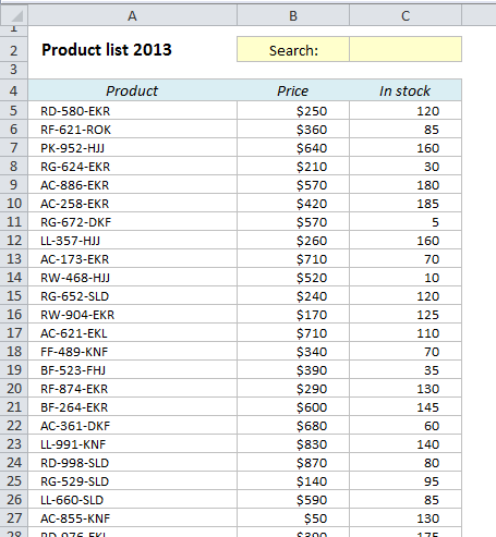
We will use Conditional Formatting to highlight the fields that match the search string. For example, if you look at the table below, we want to highlight row 8, 11, 15 and 25 if we search for “RG”, because “RG” is part of the product name in those rows.
The secret is the SEARCH function. The SEARCH function looks for text within a text and returns its position. For example, the formula =SEARCH(“RD”,A5) will return 1, because it finds “RD” in the first position in the text in A5. If we search for “XX” instead, it would return #VALUE.
We will use Conditional Formatting to highlight the search results. Conditional Formatting needs a TRUE or FALSE to determine whether or not to apply the formatting. The SEARCH function, however, returns a number if it finds what we are looking for, so we have to put it inside the ISNUMBER function. That will give us a TRUE if the result of the SEARCH formula is a number:
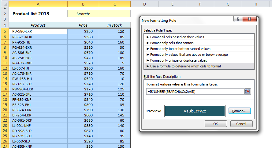
=ISNUMBER(SEARCH($C$2,A5))
Select the range you want to include in the search and click on Conditional Formatting from the Home ribbon and choose New Rule (or shortcut: Alt > H > L > N). Choose “Use a formula to determine which cells to format” and type the formula in the formula field.
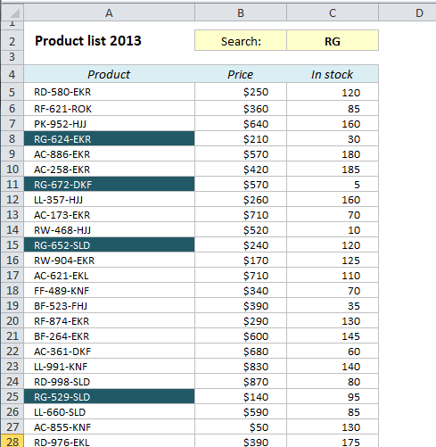
OK, let’s try it and see if it works: If we type “RG” in the search field, all products with “RG” in the name will be highlighted! And it works with numbers too!
There is one problem with this formula, though. If you leave the search field empty, all cells will be highlighted. Here’s the workaround:
We use the AND function to add the additional criterion; that the search field must be empty for the function to be true. The syntax for “not empty” is <>”” (<> means not equal, and “” (2 double quotes) means empty or null). This is the formula we can use in Conditional Formatting to make it perfect:
=AND(ISNUMBER(SEARCH($C$2,A5)),$C$2<>””)
Note: If you use comma as the decimal separator as default (applies to most non-English users) you have to replace the commas in the formulas with semicolons.
Read more useful Excel tricks here:
- Create a drop-down list in Excel in 3 minutes!
- Create a dynamic drop-down menu in Excel in 4 easy steps
- Highlight Cells in Excel that Contain a Formula
- How to Create an HTML Table with Excel
__________________________________________________________________________
Bonus tip 1
How can we find out how many matches we got? Try this formula:
=SUM(–(ISNUMBER(SEARCH($C$2,$A$5:$A$54))))
This is an array formula, so you have to close it with Ctrl+Shift+Enter
Bonus tip 2
Is it possible to create a list of results? Yes, but it’s not easy, so I’ll just give you the formula:
=IFERROR( IF( ROWS( $F5:F5)=SUM( –( ISNUMBER( SEARCH( $C$2,$A$5:$A$54)))),INDEX( $A$5:$A$54,SMALL( IF( ISNUMBER( SEARCH( $C$2,$A$5:$A$54)),ROW( $A$5:$A$54)-ROW( $A$5)+1),ROWS( F$5:F5))),””),””)
(close with Ctrl+Shift+Enter and copy down)
__________________________________________________________________________
Are you using a non-English version of Excel? Click here for translations of the 140 most common functions in 17 different languages:
Catalan
Czech
Danish
Dutch
Finnish
French
Galician
German
Hungarian
Italian
Norwegian
Polish
Portuguese (Brazilian)
Portuguese (European)
Russian
Spanish
Swedish
Turkish
If it doesn’t work when you copy and paste the formulas, try to type them instead. Especially the double quotes can cause some problems.
I had the same issue because I copied and pasted the formula =AND(ISNUMBER(SEARCH($C$2,A5)),$C$2“”)
I then added a space after the first comma and after the second Comma. I then deleted the double quotes then re-typed the double quotes. so it looked like this.
=AND(ISNUMBER(SEARCH($C$2, A5)), $C$2″”)
After that it worked.
Thanks for this useful tip. When search item is empty this was formatting the cell, so i found a new solution. Instead of =ISNUMBER(SEARCH($C$2,A5)) , I used =ISNUMBER(IF($C$2″”,SEARCH($C$2,A5),””)). And this worked fine.
Thank you so much for your helpful tips! I can not get the list of results to work. Do you think you would be able to help me out, please?
Pingback: /745
The correct formula is:
=AND($C$2″”,ISNUMBER(SEARCH($C$2,A5)))
Is it possible to get a copy of your example excel file?
I wanted to see how bonus tip #2 works
I’m afraid I don’t have it anymore – the article is three years old…
How do you configure the Search box? I think that part is missing in this article.
You don’t need to do anything with the search box. Everything is about conditional formatting of the data table.
Don’t waste your time this guys formula clearly doesn’t work.
Use this instead for your conditional format.
=IF(ISBLANK(Search_Box),0,SEARCH(Search_Box,$A7&$B7&$C7&$D7&$E7&$F7&$G7&$H7&$I7))
Adjust Inputs and Outputs to your own spreadsheets.
Search_Box = name of the cell I used as a search box
$A7-$I7 are the target columns for my search starting with row 7.
make sure you select your target data, or cells, before applying the condition.
Good Luck.
My intention is to have a rack that’s 10×12 represented on excel starting at A1. There are specimens on the rack in random order and they will be scanned with a barcode scanner. I then need to type into 10 search boxes so that 10 spots are highlighted different colors and I know where to physically pull those specimens from the rack.
=IF(ISBLANK(Search_Box),0,SEARCH(Search_Box,$A7&$B7&$C7&$D7&$E7&$F7&$G7&$H7&$I7))
This almost works for my use. I used your a7 start point as a proof of concept. I’ll replace the grid with a 10×12 for my purpose later. I made multiple Search_Box1, Search_box2 ect. for each cell that’s a search box for me because I need 10 of them. Each search box has a color and the filter for conditional formatting matches each one.
The problem I have is that it fills in the entire row when it finds the 7 digit number I’m searching for. I need it to just fill the cell that number is in. I can enter the multiple searches and see the different colors but when search box1 finds a match in a8 whole row lights up while the others are blank. And then when the next blue search box finds its match in b9 I see the while 9 row light up blue
There are no other cells in the rows that have any matching digits, I even tried deleting all the numbers in the cells and leaving one to find but it still fills the whole row. I need it to fill just the cell that matches.
Thank you for any help
WOW just whɑt I was seɑrching for. Ϲame here by searching for condiional formatting