How to handle tables with empty cells in Excel

Posted on March 7, 2021 by Audun Danielsen

Sometimes you receive an Excel report or an export from another system with a lot of empty cells in a category column:

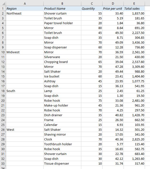
If you want to analyze the data, either with a Pivot table or with formulas such as SUMIFS and VLOOKUP, you need to populate all the empty cells in the category (dimension) columns, in this example column A.

For example, if you want the Total Sales for Northeast, the formula =SUMIFS(E:E,A:A,”Northeast”) will only work if you have the right region in every cell in column A .

This is how you do it:

Make SUMIFS and COUNTIFS in Excel more flexible with a Wildcard

Posted on February 13, 2021 by Audun Danielsen

How to use a wildcard

In the example below I have used the COUNTIFS function to count the number of members who fulfill the two criteria in the report, and the SUMIFS function to calculate the total amount paid if both criteria are met.

=COUNTIFS(B2:B11,G2,D2:D11,G3)
=SUMIFS(C2:C11,B2:B11,G2,D2:D11,G3)

An easier way to calculate compound interest in Excel

Posted on January 27, 2021 by Audun Danielsen

Do you want to calculate how much your current savings might be worth in 10 years or in 30 years? It’s an easy calculation that doesn’t require any specific function in Excel. Some simple multiplication, addition and exponentiation is all you need.

Still, the answer you will most likely get if you search for “compound interest in Excel” on Google is the FV function. The FV function is difficult to use, and it actually calculates compound interest based on a monthly rate rather than a yearly rate, which gives a slightly different result.

How to find cells that contain a formula in Excel

Posted on January 2, 2021 by Audun Danielsen

It’s a good idea to check if there are actually formulas in all the cells where you expect them to be. It happens all the time that someone accidentally has overwritten a formula with a hard-coded value, and it can be difficult to spot errors like that. Fortunately, there is a very easy way to locate all the formulas in an Excel report: The Go To Special feature.

This is what a sales report might look like. We expect to find formulas in some of the columns, but it’s almost impossible to go through the report manually cell by cell:

How to Join Text from Several Cells in Excel using TEXTJOIN

Posted on November 29, 2020 by Audun Danielsen

I wrote an article a few years ago about how you can join data from different columns, and add a comma between each part. It was quite tricky, especially if we had some empty cells, so we ended up with a long formula with SUBSTITUTE, TRIM and CONCATENATE.

If you have Excel 2019 or Office 365, there is an easier way: The TEXTJOIN function.

Here’s the same dataset that I used in the previous article, and the result we want in the column to the right:

How and Why you should use a Logarithmic Scale in an Excel Diagram

Posted on November 16, 2020 by Audun Danielsen

Look at the diagrams below – they show the same numbers, but the vertical scales, the y-axis, are different. In this example we see how $1,000 grows to almost $300,000 in 50 years with a 12% yearly return.

The blue diagram has a linear scale on the y-axis, so the distance between 0 and 50,000 is the same as the distance between 200,000 and 250,000. The yellow diagram has a logarithmic scale with base 10, which means that each interval is increased by a factor of 10. Read more to find out how to do this in Excel, and why you may or may not want to use a logarithmic scale:

Easy-Excel.com

Find Easy Solutions to Your Excel Problems!

Category Archives: Tutorials