This is a very useful trick if you have a report showing dates and budget figures, and you want to make it more readable by making the future dates less visible.
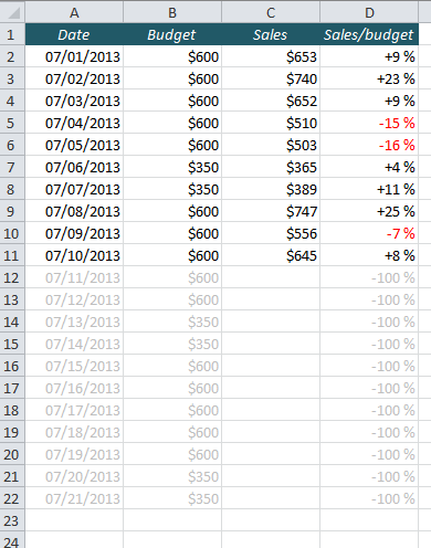
Take a look at the report to the right. Assuming today’s date is 7/10, we want the dates from 7/1 through 7/10 to be easy to read, while the dates in the future should be hidden or greyed out. The trick is to not only dim the dates, but also the other columns on the same rows. This is an easy trick that you can apply on any report you get your hands on! Here’s how to do it:
We will use Conditional Formatting with a formula to change the font colour to grey for the dates in the future. Conditional Formatting checks whether a statement is TRUE og FALSE. For each row we want to check if the date is greater that today’s date, and we want to use just one formula for the whole table.
For the first data row in the table the formula =A2>TODAY() would check the date. The formula for the second row would be =A3>TODAY(), for the third row =A4>TODAY() and so on.
As we see, the only thing that changes is the row reference (2, 3, and 4), whereas the column reference, A, stays the same. Thus, in order to make it work for the whole table at once we have to lock the column reference with a dollar sign, and leave the row reference without it: =$A2>TODAY().
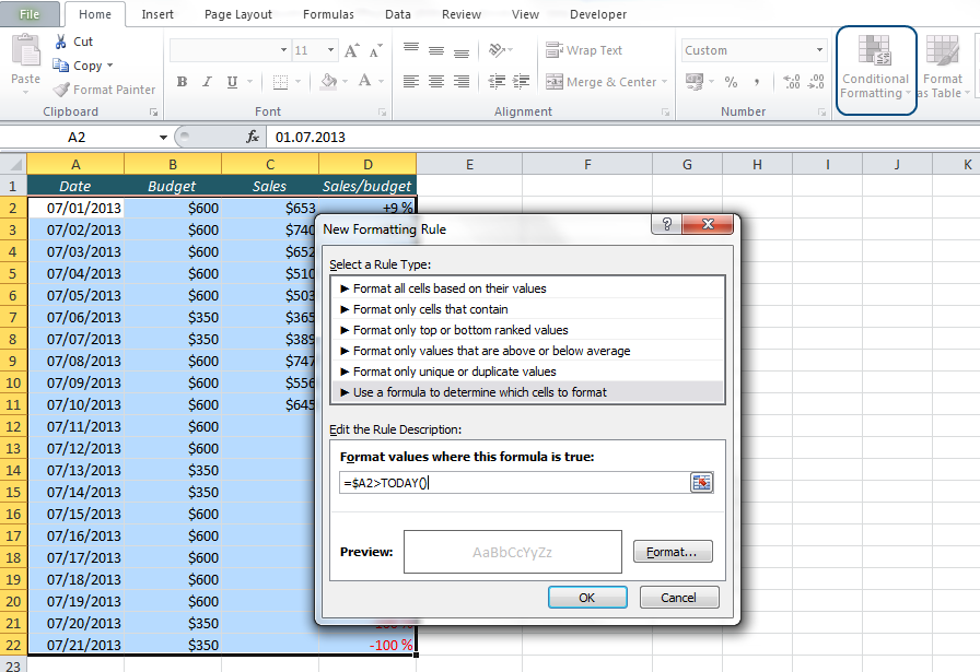
Let’s do it: Select the whole table and choose Conditional Formatting from the Home ribbon, then select New Rule. Select “Use a formula to determine which cells to format” and type the formula into the field below. Finally, click the Format button to choose font colour.
Because we are using the TODAY function, Excel will always check the current date, so when you open the same report tomorrow, one more row will be visible.
More on Conditional Formatting:
- Highlight an Entire Row in Excel Based on One Cell Value
- The Easiest Way to Hide Zeros in Excel
- Create a Search Box in Excel without VBA
Are you using a non-English version of Excel? Click here for translations of the 140 most common functions in 17 different languages:
Catalan
Czech
Danish
Dutch
Finnish
French
Galician
German
Hungarian
Italian
Norwegian
Polish
Portuguese (Brazilian)
Portuguese (European)
Russian
Spanish
Swedish
Turkish
This tutorial was really helpful, but what if you need to conditionally highlight everything before “Today” at 9:00am? I have a document with time formats like “4/17/2014 4:08:00 PM” and I need to highlight everything with a value of today’s date before 9am.
The formula =TODAY() returns a serial number, e.g. 41765 for May 6th, 2014. For every hour you can add 1/24 to this number, so in order to highlight “Today at 9:00 AM”, you can use this formula in Conditional Formatting:
=$A2>TODAY()+9/24