In the newer versions of Excel (2019 and 365) you can finally extract unique values with one simple function: UNIQUE. In previous versions, you either had to do it manually with the advanced filter, with a pivot table, or with a super-complicated formula that was impossible to remember.
Now it’s easy: Just use the UNIQUE function!
UNIQUE is one of the new Spill functions in Excel, which means that you type the formula in a cell, e.g. D2, and it populates as many cells below as it needs. So keep in mind that you need to have a sufficient number of empty cells to make room for the results.
Here’s how you do it:
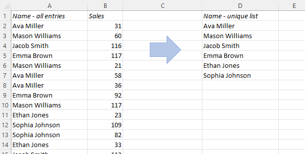
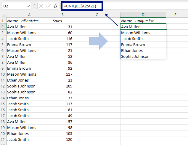
In this example, I have a list of transactions. There are 20 rows of data, but we only have six unique sales reps, so I want to create a small table with one row for each rep. This formula is all I need:
=UNIQUE(A2:A26)
It will find the unique values and spill down automatically. We don’t even have to copy down!
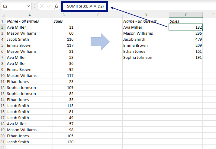
To add sales figures per sales rep, just use the SUMIFS:
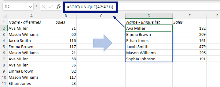
If you want the names in alphabetical order, you can wrap the SORT function around the UNIQUE function:
=SORT(UNIQUE(A2:A26))
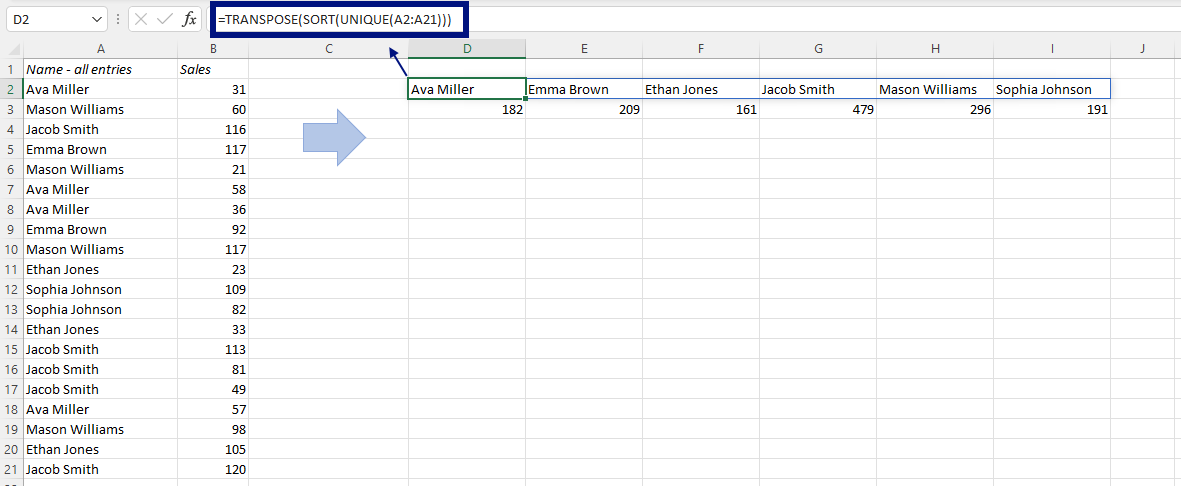
And if you want the names as column header, you can wrap the TRANSPOSE function around SORT and UNIQUE:
=TRANSPOSE(SORT(UNIQUE(A2:A26)))
More Excel Tricks:
Sum across multiple sheets in Excel
Make SUMIFS and COUNTIFS more flexible with a Wildcard
Summarize a whole table in Excel without writing a formula
Are you using a non-English version of Excel? Click here for translations of the 140 most common functions in 17 different languages:
Catalan
Czech
Danish
Dutch
Finnish
French
Galician
German
Hungarian
Italian
Norwegian
Polish
Portuguese (Brazilian)
Portuguese (European)
Russian
Spanish
Swedish
Turkish
I’m afraid it works only in 365, I have 2019 plus professional and cannot use this function 🙁