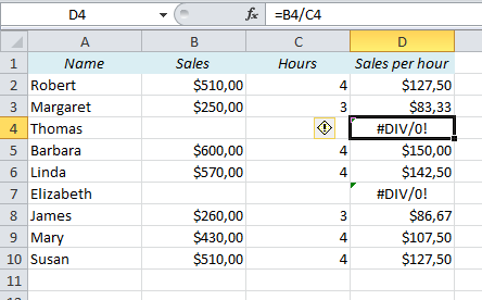
What does the error message #DIV/0 mean? Take a look at this table. It’s a sales report, with the total sales in column B, the number of hours in column C, and finally Sales per hour in column D.

Sales per hour is the total sales divided by the number of hours, and if the Hours field is empty, we are basically telling Excel to divide something by zero. Obviously, that’s impossible, and Excel returns an error message: #DIV/0.

The error message is there for a very good reason, but if we want to show this report to someone else, it would definitely look a lot better if it wasn’t there. Let’s see what we can do about it:

I’ve seen many people solve this problem simply by deleting the cells that return an error message, but that’s only curing the symptoms. If you do that, the report won’t update correctly if you change the numbers in column B and C, so we have to find a better way.

The solution is the IFERROR function. It let’s you replace the error message (#DIV/0, #N/A, #VALUE etc.) with something else, e.g. a dash, a null string, a zero, or a text. Here’s how it works:

The formula in D4 is =B4/C4. If we want to return a dash instead of the error message, we use this formula: =IFERROR(B4/C4,”-“). The formula returns whatever is between the double quotes if the original calculation (B4/C4) returns an error message.

Note: If you want to return a number, you don’t need the double quotes. It would look like this: =IFERROR(B4/C4,0)

Other Easy Excel Tricks:

• The Easiest Way to Hide Zeros in Excel
• Convert text to numbers in Excel using formulas
• Highlight Cells in Excel that Contain a Formula

Are you using a non-English version of Excel? Click here for translations of the 100 most common functions.