Creating a drop-down menu in Excel may look difficult, but it’s actually super easy! It won’t take you more than 3 minutes the first time you do it, and when you get the hang of it, it only takes a few seconds!
Just follow these 3 steps to create a drop-down list in Excel:
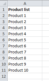
1. Create a list of the items that you want to appear in the drop-down menu.
2. Name the list.
Select the range and press Ctrl+Shift+F3 to open the name manager. If the list has a headline (it should!), choose Top row.

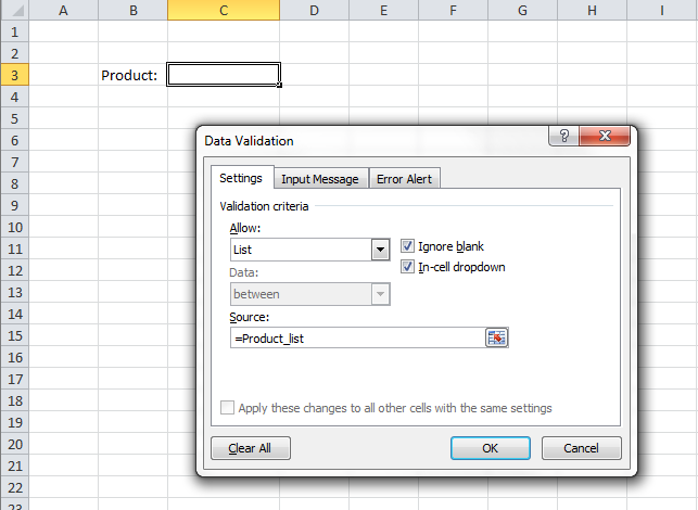
3. Create the drop-down menu.
Now you can create a drop-down menu anywhere you want in the workbook. Select a cell and press Alt, then D, then L to open the Data Validation window. Choose List in the first field.
In the source field, simply press F3 to retrieve your list names and choose the one you want for this drop-down.
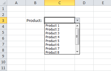
Done!
Note: If you want to create many drop-down menus in one workbook, it might be a good idea to create all the lists in one tab.
Read also:
Create a dynamic drop-down menu in Excel in 4 easy steps
Here’s a video I made that shows you how easy it is (in Norwegian, 1 minute): http://www.youtube.com/watch?v=V20I4osy8mc&feature=plcp
Are you using a non-English version of Excel? Click here for translations of the 100 most common functions.